Stata-like analysis of unstratified matched-case control data

Using data from vectors, data from a 2x2 contingency table, or individual cell counts, mcc() and mcci() will calculate McNemar's \(\chi^{2}\); point estimates and confidence intervals for the difference, ratio, and relative difference of proportion of pairs with the exposure; and the odds ratio with a confidence interval.

Usage

mcc(cases = NULL, controls = NULL, table = NULL, conf_level = 0.95)

mcci(a, b, c, d, conf_level = 0.95)

Arguments

cases, controls

Numeric vectors of the same length, with values of 0 (unexposed) and 1 (exposed). The default for these variables is NULL, and an error will be thrown if you attempt to provide these parameters as well as table. If provided, these variables are used to construct a 2x2 matrix in the same format as table.

table

A 2x2 integerish (see checkmate::check_integerish()) matrix with matched case-control data. The default value of table is NULL, and an error will be thrown if you provide table as well as cases and controls.

The table should have the following format, where each cell represents a pair of a matched case and control:

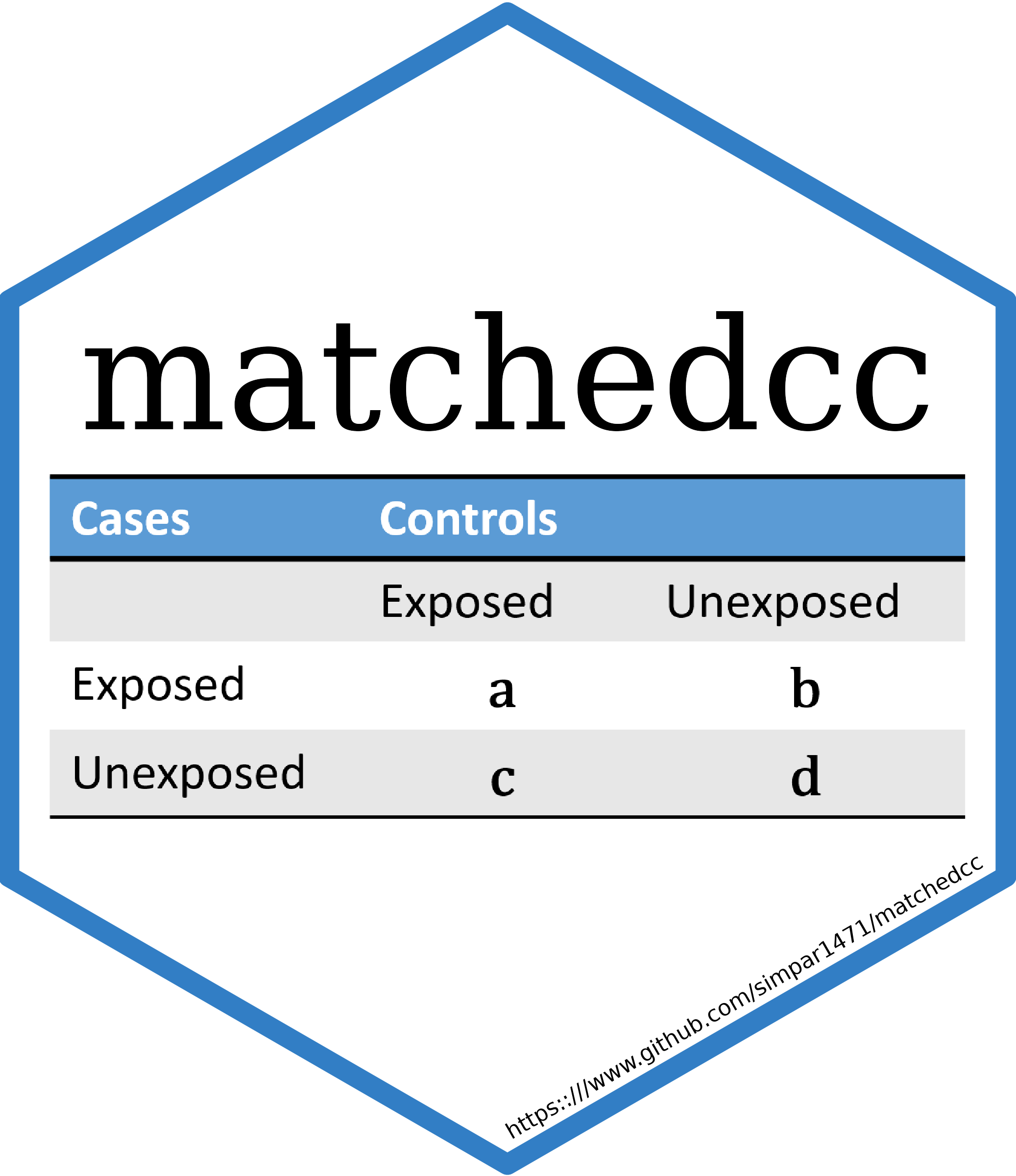
Cases	Controls
	Exposed	Unexposed
Exposed	a	b
Unexposed	c	d

conf_level

Numeric scalar from 0.1 to 0.9999. Controls level at which to calculate confidence intervals. Default = 0.95 (95% confidence intervals).

a, b, c, d

Single integerish values with cell counts that correspond to a 2x2 table of matched case control data.

Value

A named list with 5 elements:

data

A 3x3 matrix generated using the data provided, formatted for matched case-control analysis and with row/column totals.

mcnemar_chi2

Results from analysing the matched case-control data with mcnemar.test(), without Yates' continuity correction.

mcnemar_exact_p

Result of an exact test of \({H}_{0}\): \(OR = 1\), calculated using the binomial distribution.

proportions

A two-element numeric vector with the proportion of of cases and controls with the exposure.

statistics

A 4 row, 3 column numeric matrix with point estimates and confidence intervals for the ratio, difference, and relative difference in the proportion of cases/controls with the exposure, and the odds ratio.

References

Exact Chi-squared statistic:
McNemar, Q. (1947) Note on the sampling error of the difference between correlated proportions or percentages Psychometrika 12(2): 153–157. doi:10.1007/bf02295996

Other steps:
Agresti, A. (2013) Categorical Data Analysis 3rd ed. Hoboken, NJ: Wiley. pp. 414-417.

Examples

data <- matchedcc::mccxmpl
mcc(cases = data$case, controls = data$control)
#> $data
#>            Controls
#> Cases       Unexposed Exposed Total
#>   Unexposed         8       8    16
#>   Exposed           3       8    11
#>   Total            11      16    27
#> 
#> $mcnemar_chi2
#> 
#> 	McNemar's Chi-squared test
#> 
#> data:  mcc_table
#> McNemar's chi-squared = 2.2727, df = 1, p-value = 0.1317
#> 
#> 
#> $mcnemar_exact_p
#> Exact McNemar significance probability 
#>                              0.2265625 
#> 
#> $proportions
#>   Proportion with factor
#>        Cases  Controls
#>    0.5925926 0.4074074
#> 
#> $statistics
#>             estimate [95% CI]
#> statistic     estimate       lower      upper
#>   difference 0.1851852 -0.08225420  0.4526246
#>   ratio      1.4545455  0.89110096  2.3742568
#>   rel. diff. 0.3125000 -0.02436881  0.6493688
#>   odds ratio 2.6666667  0.64003641 15.6064036
#> 

# Convert data into 2x2 table
data$case_fctr <- factor(data$case, levels = c(1, 0),
                         labels = c("6+ cups", "0 cups"))
data$control_fctr <- factor(data$control, levels = c(1, 0),
                            labels = c("6+ cups", "0 cups"))
mcc(table = table(data$control_fctr, data$case_fctr))
#> $data
#>            Controls
#> Cases       Unexposed Exposed Total
#>   Unexposed         8       3    11
#>   Exposed           8       8    16
#>   Total            16      11    27
#> 
#> $mcnemar_chi2
#> 
#> 	McNemar's Chi-squared test
#> 
#> data:  mcc_table
#> McNemar's chi-squared = 2.2727, df = 1, p-value = 0.1317
#> 
#> 
#> $mcnemar_exact_p
#> Exact McNemar significance probability 
#>                              0.2265625 
#> 
#> $proportions
#>   Proportion with factor
#>        Cases  Controls
#>    0.4074074 0.5925926
#> 
#> $statistics
#>             estimate [95% CI]
#> statistic      estimate       lower     upper
#>   difference -0.1851852 -0.45262457 0.0822542
#>   ratio       0.6875000  0.42118444 1.1222073
#>   rel. diff. -0.4545455 -1.16725963 0.2581687
#>   odds ratio  0.3750000  0.06407626 1.5624111
#> 

# Alternatively, provide cell counts to `mcci()`
table <- table(data$control_fctr, data$case_fctr)
mcci(a = table[1,1],
     b = table[1,2],
     c = table[2,1],
     d = table[2,2])
#> $data
#>            Controls
#> Cases       Unexposed Exposed Total
#>   Unexposed         8       3    11
#>   Exposed           8       8    16
#>   Total            16      11    27
#> 
#> $mcnemar_chi2
#> 
#> 	McNemar's Chi-squared test
#> 
#> data:  mcc_table
#> McNemar's chi-squared = 2.2727, df = 1, p-value = 0.1317
#> 
#> 
#> $mcnemar_exact_p
#> Exact McNemar significance probability 
#>                              0.2265625 
#> 
#> $proportions
#>   Proportion with factor
#>        Cases  Controls
#>    0.4074074 0.5925926
#> 
#> $statistics
#>             estimate [95% CI]
#> statistic      estimate       lower     upper
#>   difference -0.1851852 -0.45262457 0.0822542
#>   ratio       0.6875000  0.42118444 1.1222073
#>   rel. diff. -0.4545455 -1.16725963 0.2581687
#>   odds ratio  0.3750000  0.06407626 1.5624111
#>